

pandas Basics
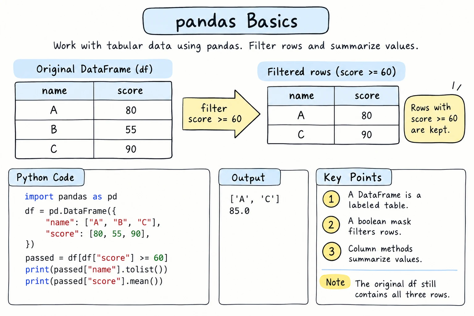
What you'll learn
- How to add computed columns and sort rows
- How to count values and summarize groups with
groupby,agg, andpivot_table - How to clean a table (
drop_duplicates,rename,drop) and combine tables withconcatandmerge - How to work with text (
.str) and dates (.dt) in whole columns - When to use
apply, why vectorized operations are usually better, and how to avoid chained indexing
Why it matters
In Reading Data Files, you loaded tables and picked out rows. The real value of pandas comes next: answering questions. "Which city earned the most?", "What is the average order per product each month?", "Which customers from Samarkand bought juice?" Each of these would take a loop and a dictionary of totals in plain Python. In pandas, each is one or two lines, and the same code works for 10 rows or 10 million.
The sales data
Most examples in this lesson use the same small table of shop sales. It is created from text with io.StringIO, so every example runs on its own:
import io
import pandas as pd

text = """date,city,product,quantity,price
2026-01-05,Tashkent,Tea,4,15000
2026-01-12,Samarkand,Samsa,10,8000
2026-01-20,Tashkent,Juice,3,12000
2026-02-03,Bukhara,Tea,5,15000
2026-02-14,Tashkent,Samsa,12,8000
2026-02-21,Samarkand,Juice,6,12000
2026-03-02,Bukhara,Samsa,8,8000
2026-03-10,Tashkent,Tea,7,15000
2026-03-18,Samarkand,Tea,2,15000
2026-03-25,Bukhara,Juice,4,12000
"""
sales = pd.read_csv(io.StringIO(text), parse_dates=["date"])
print(sales) date city product quantity price
0 2026-01-05 Tashkent Tea 4 15000
1 2026-01-12 Samarkand Samsa 10 8000
2 2026-01-20 Tashkent Juice 3 12000
3 2026-02-03 Bukhara Tea 5 15000
4 2026-02-14 Tashkent Samsa 12 8000
5 2026-02-21 Samarkand Juice 6 12000
6 2026-03-02 Bukhara Samsa 8 8000
7 2026-03-10 Tashkent Tea 7 15000
8 2026-03-18 Samarkand Tea 2 15000
9 2026-03-25 Bukhara Juice 4 12000parse_dates=["date"] converts the date column while reading, which saves a separate pd.to_datetime() call.
Computed columns
Assigning to a new column name creates that column. The math runs on every row at once, with no loop:
import io
import pandas as pd

text = """date,city,product,quantity,price
2026-01-05,Tashkent,Tea,4,15000
2026-01-12,Samarkand,Samsa,10,8000
2026-02-03,Bukhara,Tea,5,15000
"""
sales = pd.read_csv(io.StringIO(text))

sales["revenue"] = sales["quantity"] * sales["price"]
sales["big_order"] = sales["revenue"] >= 75000
print(sales)
print()
print("Total:", sales["revenue"].sum()) date city product quantity price revenue big_order
0 2026-01-05 Tashkent Tea 4 15000 60000 False
1 2026-01-12 Samarkand Samsa 10 8000 80000 True
2 2026-02-03 Bukhara Tea 5 15000 75000 True
Total: 215000This style, where one operation works on a whole column, is called a vectorized operation. It is shorter than a loop and much faster, because pandas does the looping in optimized compiled code.
Sorting
sort_values() sorts by one or more columns. ascending=False gives the largest first:
import io
import pandas as pd

text = """city,product,quantity,price
Tashkent,Tea,4,15000
Samarkand,Samsa,10,8000
Tashkent,Juice,3,12000
Bukhara,Tea,5,15000
Tashkent,Samsa,12,8000
"""
sales = pd.read_csv(io.StringIO(text))
sales["revenue"] = sales["quantity"] * sales["price"]

print(sales.sort_values("revenue", ascending=False))
print()
print(sales.sort_values(["city", "revenue"], ascending=[True, False])) city product quantity price revenue
4 Tashkent Samsa 12 8000 96000
1 Samarkand Samsa 10 8000 80000
3 Bukhara Tea 5 15000 75000
0 Tashkent Tea 4 15000 60000
2 Tashkent Juice 3 12000 36000
city product quantity price revenue
3 Bukhara Tea 5 15000 75000
1 Samarkand Samsa 10 8000 80000
4 Tashkent Samsa 12 8000 96000
0 Tashkent Tea 4 15000 60000
2 Tashkent Juice 3 12000 36000The second sort orders cities alphabetically, then revenue from high to low inside each city. Notice that the index labels travel with their rows. Add .reset_index(drop=True) if you want a fresh 0, 1, 2, ... index. For just the top rows, sales.nlargest(3, "revenue") is a handy shortcut.
Counting with value_counts
value_counts() counts how often each value appears, like collections.Counter:
import io
import pandas as pd

text = """city,product
Tashkent,Tea
Samarkand,Samsa
Tashkent,Juice
Bukhara,Tea
Tashkent,Samsa
Samarkand,Juice
"""
sales = pd.read_csv(io.StringIO(text))

print(sales["city"].value_counts())
print()
print(sales["city"].value_counts(normalize=True).round(2))city
Tashkent 3
Samarkand 2
Bukhara 1
Name: count, dtype: int64
city
Tashkent 0.50
Samarkand 0.33
Bukhara 0.17
Name: proportion, dtype: float64normalize=True gives shares instead of counts: half of the orders came from Tashkent.
Grouping with groupby
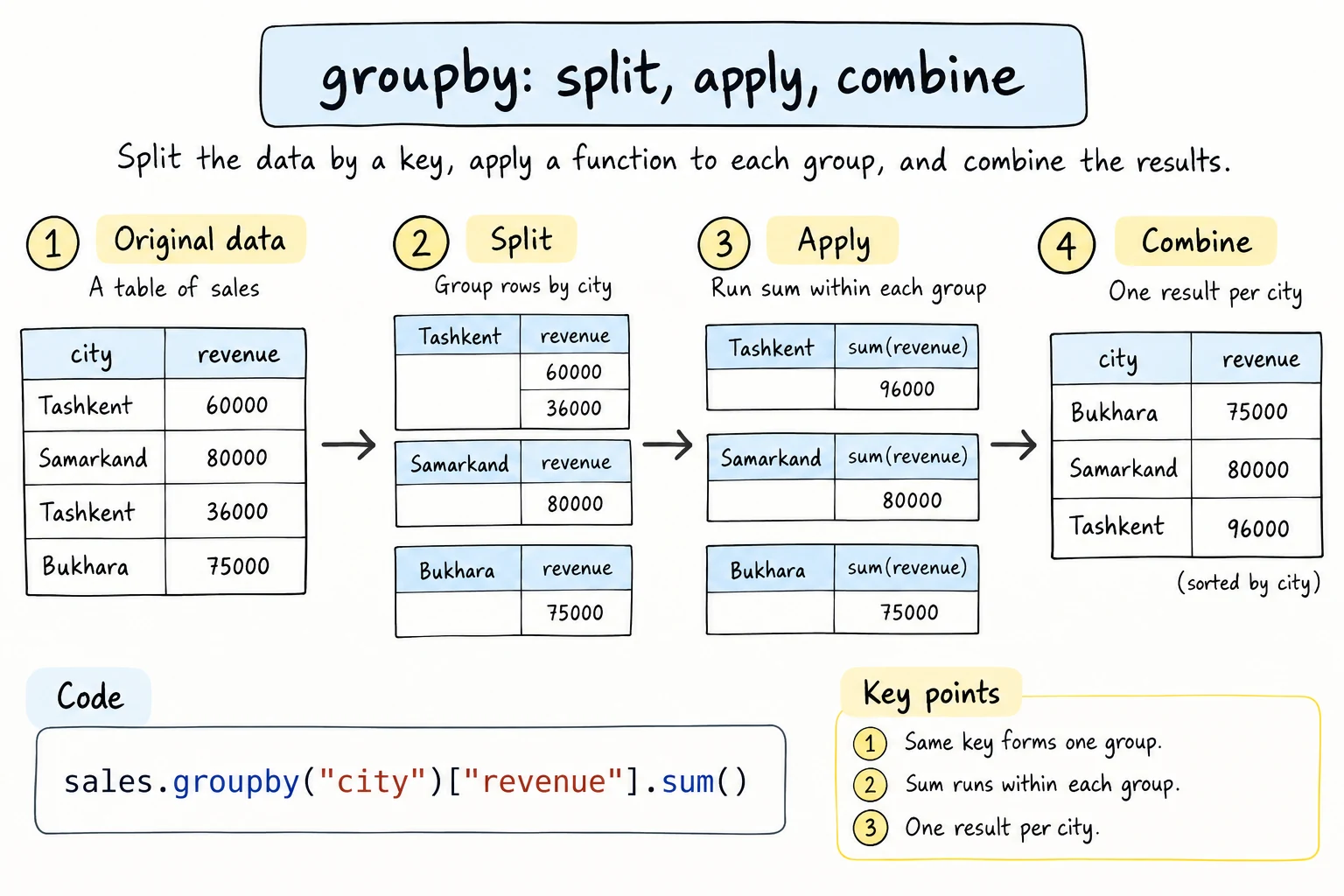
groupby answers "for each X, what is Y?". It works in three steps: split the rows into groups, apply a calculation to each group, and combine the results.
original rows       split into groups      apply: sum     combine
Tashkent   60000    Bukhara    75000   ->  75000          Bukhara    75000
Samarkand  80000    Samarkand  80000   ->  80000          Samarkand  80000
Tashkent   36000    Tashkent   60000                      Tashkent   96000
Bukhara 75000 Tashkent 36000 -> 96000import io
import pandas as pd
text = """date,city,product,quantity,price
2026-01-05,Tashkent,Tea,4,15000
2026-01-12,Samarkand,Samsa,10,8000
2026-01-20,Tashkent,Juice,3,12000
2026-02-03,Bukhara,Tea,5,15000
2026-02-14,Tashkent,Samsa,12,8000
2026-02-21,Samarkand,Juice,6,12000
2026-03-02,Bukhara,Samsa,8,8000
2026-03-10,Tashkent,Tea,7,15000
2026-03-18,Samarkand,Tea,2,15000
2026-03-25,Bukhara,Juice,4,12000
"""
sales = pd.read_csv(io.StringIO(text), parse_dates=["date"])
sales["revenue"] = sales["quantity"] * sales["price"]
print(sales.groupby("city")["revenue"].sum())
print()
print(sales.groupby("product")["quantity"].mean())
print()
print(sales.groupby("city").size())city
Bukhara 187000
Samarkand 182000
Tashkent 297000
Name: revenue, dtype: int64
product
Juice 4.333333
Samsa 10.000000
Tea 4.500000
Name: quantity, dtype: float64
city
Bukhara 3
Samarkand 3
Tashkent 4
dtype: int64The pattern is always df.groupby(key)[column].calculation(). The result is a Series whose index is the group names, sorted alphabetically. .size() counts rows per group. .count() also exists, but it counts non-missing values in each column.
Several calculations at once with agg
agg() runs several aggregations in one go. Named aggregations let you choose the output column names:
import io
import pandas as pd

text = """city,product,quantity,price
Tashkent,Tea,4,15000
Samarkand,Samsa,10,8000
Tashkent,Juice,3,12000
Bukhara,Tea,5,15000
Tashkent,Samsa,12,8000
Samarkand,Juice,6,12000
Bukhara,Samsa,8,8000
Tashkent,Tea,7,15000
Samarkand,Tea,2,15000
Bukhara,Juice,4,12000
"""
sales = pd.read_csv(io.StringIO(text))
sales["revenue"] = sales["quantity"] * sales["price"]

summary = sales.groupby("city").agg(
    orders=("revenue", "count"),
    total=("revenue", "sum"),
    average=("revenue", "mean"),
    biggest=("quantity", "max"),
)
print(summary.sort_values("total", ascending=False).round(1)) orders total average biggest
city
Tashkent 4 297000 74250.0 12
Bukhara 3 187000 62333.3 8
Samarkand 3 182000 60666.7 10Each argument reads as new_name=(column, calculation). Grouping by two columns, such as groupby(["city", "product"]), gives one row per combination.
Group totals back on every row
Two more tools often appear next to groupby in real reports. idxmax() returns the label of the largest value (which city, not how much), and transform("sum") returns each group's total on every row of that group, so you can compute shares:
import io
import pandas as pd

text = """city,quantity,price
Tashkent,4,15000
Samarkand,10,8000
Tashkent,3,12000
Bukhara,5,15000
"""
sales = pd.read_csv(io.StringIO(text))
sales["revenue"] = sales["quantity"] * sales["price"]

by_city = sales.groupby("city")["revenue"].sum()
print(by_city.idxmax(), by_city.max())

sales["city_share"] = sales["revenue"] / sales.groupby("city")["revenue"].transform("sum")
print(sales[["city", "revenue", "city_share"]].round(2))Tashkent 96000
city revenue city_share
0 Tashkent 60000 0.62
1 Samarkand 80000 1.00
2 Tashkent 36000 0.38
3 Bukhara 75000 1.00Pivot tables
A pivot table spreads one grouping across the rows and another across the columns, like a spreadsheet summary:
import io
import pandas as pd

text = """city,product,quantity,price
Tashkent,Tea,4,15000
Samarkand,Samsa,10,8000
Tashkent,Juice,3,12000
Bukhara,Tea,5,15000
Tashkent,Samsa,12,8000
Samarkand,Juice,6,12000
Bukhara,Samsa,8,8000
Tashkent,Tea,7,15000
Samarkand,Tea,2,15000
Bukhara,Juice,4,12000
"""
sales = pd.read_csv(io.StringIO(text))
sales["revenue"] = sales["quantity"] * sales["price"]

table = sales.pivot_table(
    index="city",
    columns="product",
    values="revenue",
    aggfunc="sum",
    fill_value=0,
    margins=True,
)
print(table)product Juice Samsa Tea All
city
Bukhara 48000 64000 75000 187000
Samarkand 72000 80000 30000 182000
Tashkent 36000 96000 165000 297000
All 156000 240000 270000 666000fill_value=0 fills combinations with no sales, and margins=True adds the All row and column with totals.
Cleaning helpers
Three methods tidy a freshly loaded table. drop_duplicates() removes rows that repeat exactly (or repeat in the columns you name with subset=), rename() fixes column names, and drop() removes columns you don't need:
import pandas as pd

orders = pd.DataFrame({
    "Order ID": [101, 102, 102, 103],
    "customer": ["Aziza", "Bekzod", "Bekzod", "Dilnoza"],
    "product": ["Tea", "Samsa", "Samsa", "Tea"],
    "note": ["", "", "", "gift"],
})

clean = (
    orders.drop_duplicates()                    # drop rows that repeat exactly
    .rename(columns={"Order ID": "order_id"})   # tidy column names
    .drop(columns=["note"])                     # remove columns you don't need
)
print(clean) order_id customer product
0 101 Aziza Tea
1 102 Bekzod Samsa
3 103 Dilnoza TeaThe index keeps its old labels (0, 1, 3); add .reset_index(drop=True) when you want 0, 1, 2 again.
Combining tables
When two tables have the same columns, for example one file per month, pd.concat() stacks them:
import pandas as pd

january = pd.DataFrame({"city": ["Tashkent", "Bukhara"], "revenue": [176000, 90000]})
february = pd.DataFrame({"city": ["Tashkent", "Samarkand"], "revenue": [130000, 113000]})

print(pd.concat([january, february], ignore_index=True)) city revenue
0 Tashkent 176000
1 Bukhara 90000
2 Tashkent 130000
3 Samarkand 113000When two tables share a key column instead, merge() joins them.
Merging two tables
Here, each order has only a product name, and the product details are in a second table. merge() looks up each product, like a dictionary lookup for a whole column:
import pandas as pd

orders = pd.DataFrame({
    "order_id": [101, 102, 103, 104],
    "customer": ["Aziza", "Bekzod", "Dilnoza", "Farrukh"],
    "product": ["Tea", "Samsa", "Tea", "Halva"],
    "quantity": [2, 5, 1, 3],
})
products = pd.DataFrame({
    "product": ["Tea", "Samsa", "Juice"],
    "price": [15000, 8000, 12000],
    "category": ["drink", "food", "drink"],
})

merged = orders.merge(products, on="product", how="left")
print(merged)
print()
print(orders.merge(products, on="product")) order_id customer product quantity price category
0 101 Aziza Tea 2 15000.0 drink
1 102 Bekzod Samsa 5 8000.0 food
2 103 Dilnoza Tea 1 15000.0 drink
3 104 Farrukh Halva 3 NaN NaN
order_id customer product quantity price category
0 101 Aziza Tea 2 15000 drink
1 102 Bekzod Samsa 5 8000 food
2 103 Dilnoza Tea 1 15000 drinkThe how argument decides what happens to rows without a match:
how | Keeps |
|---|---|
"inner" (default) | only keys found in both tables |
"left" | every row of the left table, with NaN where nothing matched |
"right" | every row of the right table |
"outer" | every row from both tables |
Halva is not in the product list, so a left merge keeps Farrukh's order with NaN price, and an inner merge drops it. A left merge followed by isna() is a quick way to find such missing lookups.
Text columns: the .str accessor
String methods from String Methods and Slicing work on a whole column through .str:
import pandas as pd

customers = pd.DataFrame({
    "name": ["  aziza KARIMOVA", "Bekzod Tursunov ", "dilnoza rahimova"],
    "email": ["aziza@mail.uz", "bekzod@gmail.com", "dilnoza@mail.uz"],
})

customers["name"] = customers["name"].str.strip().str.title()
customers["domain"] = customers["email"].str.split("@").str[1]
print(customers)
print()
print(customers[customers["email"].str.contains("mail.uz", regex=False)])
print(customers["name"].str.lower().str.startswith("b").tolist()) name email domain
0 Aziza Karimova aziza@mail.uz mail.uz
1 Bekzod Tursunov bekzod@gmail.com gmail.com
2 Dilnoza Rahimova dilnoza@mail.uz mail.uz
name email domain
0 Aziza Karimova aziza@mail.uz mail.uz
2 Dilnoza Rahimova dilnoza@mail.uz mail.uz
[False, True, False].str.contains() treats its pattern as a regular expression by default, so the re syntax from Regular Expressions works there. Here regex=False makes the dot a plain dot. Methods chain naturally: .str.strip().str.title().
Date columns: the .dt accessor
Datetime columns have a .dt accessor for parts of each date. Combined with groupby, it gives monthly summaries:
import io
import pandas as pd

text = """date,city,product,quantity,price
2026-01-05,Tashkent,Tea,4,15000
2026-01-12,Samarkand,Samsa,10,8000
2026-01-20,Tashkent,Juice,3,12000
2026-02-03,Bukhara,Tea,5,15000
2026-02-14,Tashkent,Samsa,12,8000
2026-02-21,Samarkand,Juice,6,12000
2026-03-02,Bukhara,Samsa,8,8000
2026-03-10,Tashkent,Tea,7,15000
2026-03-18,Samarkand,Tea,2,15000
2026-03-25,Bukhara,Juice,4,12000
"""
sales = pd.read_csv(io.StringIO(text), parse_dates=["date"])
sales["revenue"] = sales["quantity"] * sales["price"]

sales["month"] = sales["date"].dt.month
sales["weekday"] = sales["date"].dt.day_name()
print(sales[["date", "month", "weekday"]].head(3))
print()
print(sales.groupby("month")["revenue"].sum())
print()
monthly = sales.set_index("date").resample("MS")["revenue"].sum()
print(monthly) date month weekday
0 2026-01-05 1 Monday
1 2026-01-12 1 Monday
2 2026-01-20 1 Tuesday
month
1 176000
2 243000
3 247000
Name: revenue, dtype: int64
date
2026-01-01 176000
2026-02-01 243000
2026-03-01 247000
Freq: MS, Name: revenue, dtype: int64resample("MS") groups a date index into calendar months, labeled by the month start. Unlike grouping by month number, it keeps the year and adds empty months with a total of 0. To label months as text instead, group by sales["date"].dt.strftime("%Y-%m") (the format codes from Dates and Times). monthly.pct_change() gives the change from each month to the next as a fraction (0.381 means +38.1%; the first month is NaN because it has no previous month).
apply: running your own function
When no built-in operation fits, apply() calls your function once per value:
import pandas as pd

scores = pd.DataFrame({
    "student": ["Aziza", "Bekzod", "Dilnoza", "Farrukh"],
    "score": [93, 71, 85, 58],
})

def letter(score):
    if score >= 90:
        return "A"
    if score >= 80:
        return "B"
    if score >= 60:
        return "C"
    return "F"

scores["grade"] = scores["score"].apply(letter)
print(scores) student score grade
0 Aziza 93 A
1 Bekzod 71 C
2 Dilnoza 85 B
3 Farrukh 58 Fapply is flexible, but it is really a Python loop in disguise. If a vectorized version exists, prefer it: prices["price"] * 1.12 is simpler than prices["price"].apply(lambda p: p * 1.12) and often 10 to 100 times faster on large data.
For categories based on ranges, pd.cut() is the vectorized alternative to the letter function: pd.cut(scores["score"], bins=[0, 59, 79, 89, 100], labels=["F", "C", "B", "A"], include_lowest=True). Each bin includes its right edge, so (59, 79] means 60 to 79 for whole-number scores; include_lowest=True also puts a score of exactly 0 into the first bin instead of giving NaN.
Method chaining
Because most methods return a new DataFrame, you can chain them into a readable pipeline. Wrap the chain in parentheses and put one step per line:
import io
import pandas as pd

text = """date,city,product,quantity,price
2026-01-05,Tashkent,Tea,4,15000
2026-01-12,Samarkand,Samsa,10,8000
2026-01-20,Tashkent,Juice,3,12000
2026-02-03,Bukhara,Tea,5,15000
2026-02-14,Tashkent,Samsa,12,8000
2026-02-21,Samarkand,Juice,6,12000
2026-03-02,Bukhara,Samsa,8,8000
2026-03-10,Tashkent,Tea,7,15000
2026-03-18,Samarkand,Tea,2,15000
2026-03-25,Bukhara,Juice,4,12000
"""

report = (
    pd.read_csv(io.StringIO(text), parse_dates=["date"])
    .assign(revenue=lambda d: d["quantity"] * d["price"])
    .query("product != 'Samsa'")
    .groupby("city", as_index=False)["revenue"]
    .sum()
    .sort_values("revenue", ascending=False)
)
print(report) city revenue
2 Tashkent 201000
0 Bukhara 123000
1 Samarkand 102000assign() adds a column and returns a new DataFrame. The lambda d: receives the DataFrame at that point in the chain. query() filters with a short expression string, and as_index=False keeps city as a normal column. Read the chain top to bottom like a recipe.
Try it
Change the grouping column, add another aggregation, or filter a different product.
Common mistakes
1. Using and/or to combine conditions
import pandas as pd

sales = pd.DataFrame({"city": ["Tashkent", "Bukhara"], "quantity": [4, 12]})
print(sales[sales["city"] == "Tashkent" and sales["quantity"] > 5])ValueError: The truth value of a Series is ambiguous. Use a.empty, a.bool(), a.item(), a.any() or a.all().and asks Python whether the whole Series is true, which has no single answer. Use &, |, ~, with parentheses around each condition: sales[(sales["city"] == "Tashkent") & (sales["quantity"] > 5)].
2. Chained indexing when assigning
Two sets of brackets in a row, first to filter and then to pick a column, create a temporary copy. Assigning into that copy never reaches the original:
import pandas as pd

sales = pd.DataFrame({"city": ["Tashkent", "Bukhara"], "price": [15000, 8000]})
sales[sales["city"] == "Bukhara"]["price"] = 9000    # Bad: chained indexing
print(sales)                                         # Bukhara is still 8000
pandas 3 prints a warning that begins like this (pandas 2 shows a SettingWithCopyWarning instead):
ChainedAssignmentError: A value is being set on a copy of a DataFrame or Series through chained assignment.Do the selection and the assignment in one .loc step:
import pandas as pd

sales = pd.DataFrame({"city": ["Tashkent", "Bukhara"], "price": [15000, 8000]})
sales.loc[sales["city"] == "Bukhara", "price"] = 9000    # Good
print(sales) city price
0 Tashkent 15000
1 Bukhara 90003. Changing a filtered subset without .copy()
tashkent = sales[sales["city"] == "Tashkent"]
tashkent["price"] = tashkent["price"] * 2     # Bad: SettingWithCopyWarning in pandas 2
In pandas 3 this line works without a warning: thanks to Copy-on-Write, changing tashkent never changes sales. In pandas 2 it prints a warning and leaves readers unsure what was changed. If you want an independent subset to modify, say so explicitly: tashkent = sales[sales["city"] == "Tashkent"].copy(). That works quietly in every pandas version, and it is clear that sales stays unchanged.
4. Looping over rows instead of using columns
# Bad: slow and long
totals = []
for i, row in sales.iterrows():
    totals.append(row["quantity"] * row["price"])
sales["revenue"] = totals

# Good: one vectorized line
sales["revenue"] = sales["quantity"] * sales["price"]
If you write a for loop over a DataFrame, first look for a column operation, groupby, or .str/.dt method that does the job.
Practice
1. Best-selling product
Using the table below, add a revenue column and print the products sorted by total revenue, highest first.
import pandas as pd

sales = pd.DataFrame({
    "product": ["Tea", "Samsa", "Tea", "Juice", "Samsa", "Juice"],
    "quantity": [4, 10, 5, 3, 12, 6],
    "price": [15000, 8000, 15000, 12000, 8000, 12000],
})
Solution
import pandas as pd

sales = pd.DataFrame({
    "product": ["Tea", "Samsa", "Tea", "Juice", "Samsa", "Juice"],
    "quantity": [4, 10, 5, 3, 12, 6],
    "price": [15000, 8000, 15000, 12000, 8000, 12000],
})
sales["revenue"] = sales["quantity"] * sales["price"]

print(sales.groupby("product")["revenue"].sum().sort_values(ascending=False))product
Samsa 176000
Tea 135000
Juice 108000
Name: revenue, dtype: int64A grouped result is a Series, so it uses sort_values() without a column name.
2. Email domains
Count how many users have each email domain, ignoring upper and lower case.
import pandas as pd

users = pd.DataFrame({
    "email": ["aziza@Mail.uz", "bekzod@gmail.com", "dilnoza@mail.uz",
              "farrukh@GMAIL.com", "nodira@mail.uz"],
})
Solution
import pandas as pd

users = pd.DataFrame({
    "email": ["aziza@Mail.uz", "bekzod@gmail.com", "dilnoza@mail.uz",
              "farrukh@GMAIL.com", "nodira@mail.uz"],
})

domains = users["email"].str.lower().str.split("@").str[1]
print(domains.value_counts())email
mail.uz 3
gmail.com 2
Name: count, dtype: int643. Class report
For each group, show the number of students, the average score (rounded to 1 decimal), and the highest score. Use named aggregations.
import pandas as pd

results = pd.DataFrame({
    "student": ["Aziza", "Bekzod", "Dilnoza", "Farrukh", "Nodira", "Sardor"],
    "group": ["A", "B", "A", "B", "A", "B"],
    "score": [91, 67, 84, 78, 88, 72],
})
Solution
import pandas as pd

results = pd.DataFrame({
    "student": ["Aziza", "Bekzod", "Dilnoza", "Farrukh", "Nodira", "Sardor"],
    "group": ["A", "B", "A", "B", "A", "B"],
    "score": [91, 67, 84, 78, 88, 72],
})

report = results.groupby("group").agg(
    students=("student", "count"),
    average=("score", "mean"),
    best=("score", "max"),
).round(1)
print(report) students average best
group
A 3 87.7 91
B 3 72.3 784. Orders with customer cities
Merge the two tables so each order shows the customer city, then print total spending per city. Use a left merge and fill unknown cities with "Unknown".
import pandas as pd

orders = pd.DataFrame({
    "customer_id": [1, 2, 1, 3, 4],
    "amount": [120000, 45000, 80000, 300000, 60000],
})
customers = pd.DataFrame({
    "customer_id": [1, 2, 3],
    "city": ["Tashkent", "Samarkand", "Tashkent"],
})
Solution
import pandas as pd

orders = pd.DataFrame({
    "customer_id": [1, 2, 1, 3, 4],
    "amount": [120000, 45000, 80000, 300000, 60000],
})
customers = pd.DataFrame({
    "customer_id": [1, 2, 3],
    "city": ["Tashkent", "Samarkand", "Tashkent"],
})

merged = orders.merge(customers, on="customer_id", how="left")
merged["city"] = merged["city"].fillna("Unknown")
print(merged.groupby("city")["amount"].sum())city
Samarkand 45000
Tashkent 500000
Unknown 60000
Name: amount, dtype: int64Customer 4 has no record, so the left merge gives NaN for the city, which fillna() replaces.
5. Monthly pipeline
Write a single method chain that reads the CSV text below, adds revenue, keeps only rows from Tashkent and Samarkand, adds a month column with .dt.month, and builds a pivot table of revenue with months as rows and cities as columns.
date,city,quantity,price
2026-01-05,Tashkent,4,15000
2026-01-18,Samarkand,10,8000
2026-02-03,Bukhara,5,15000
2026-02-14,Tashkent,12,8000
2026-02-21,Samarkand,6,12000
2026-03-10,Tashkent,7,15000
2026-03-18,Samarkand,2,15000
Solution
import io
import pandas as pd

text = """date,city,quantity,price
2026-01-05,Tashkent,4,15000
2026-01-18,Samarkand,10,8000
2026-02-03,Bukhara,5,15000
2026-02-14,Tashkent,12,8000
2026-02-21,Samarkand,6,12000
2026-03-10,Tashkent,7,15000
2026-03-18,Samarkand,2,15000
"""

table = (
    pd.read_csv(io.StringIO(text), parse_dates=["date"])
    .assign(revenue=lambda d: d["quantity"] * d["price"])
    .loc[lambda d: d["city"].isin(["Tashkent", "Samarkand"])]
    .assign(month=lambda d: d["date"].dt.month)
    .pivot_table(index="month", columns="city", values="revenue", aggfunc="sum")
)
print(table)city Samarkand Tashkent
month
1 80000 60000
2 72000 96000
3 30000 105000.loc also accepts a function, which lets you filter in the middle of a chain. Each lambda d: receives the DataFrame as it is at that step, so month can be added after the filter.
Recap
- New columns come from vectorized math:
df["revenue"] = df["quantity"] * df["price"];sort_values()orders rows andvalue_counts()counts values. df.groupby(key)[col].sum()summarizes groups. Useagg(name=(col, func))for several results,transform()to put group totals on every row,idxmax()for the winning label, andpivot_table()for a two-way summary.- Clean with
drop_duplicates(),rename(), anddrop(); stack same-shaped tables withconcat(); join on a key withmerge(other, on=key, how=...)(a left merge keeps every left row). .strand.dtapply string and date operations to whole columns;pct_change()turns a monthly series into growth rates.apply()runs your own function, but vectorized operations are simpler and faster when they exist.- Assign with
.loc[mask, col] = value, use.copy()for subsets you will modify, combine conditions with&and|, and keep the DataFrames that methods return.