

Project: Sales Data Report
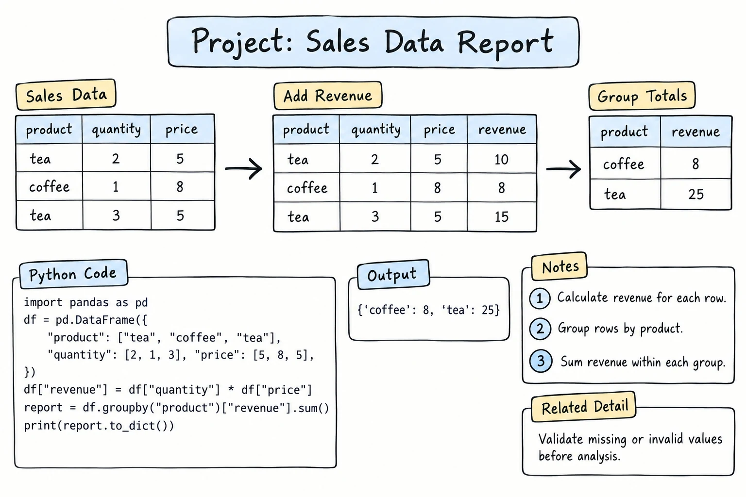
What you'll learn
- How a real data analysis flows: generate or collect, load, inspect, clean, analyze, visualize, report
- How to find and fix messy data: inconsistent text, duplicates, missing values, and wrong types
- How to answer business questions with
groupby,agg, andpivot_table - How to combine three charts into one dashboard figure and save it as a PNG
- How to write a short text summary with f-strings and save every result to files
Why it matters
A shop owner does not want a DataFrame. They want answers: "Are we growing?", "Which product earns the most?", "Is Samarkand worth a second store?" A data report turns thousands of rows into a few numbers, one picture, and a paragraph anyone can read.
In this project you do the whole job, from a raw CSV file to a finished report. Most of the work is not the charts. It is cleaning: real data always has typos, gaps, and duplicates, and a report built on dirty data is confidently wrong.
Running the code
This project needs pandas and matplotlib: python -m pip install pandas matplotlib. The outputs shown come from pandas 3. With pandas 2, text columns show the type object instead of str, dates show datetime64[ns], and a few tables may be spaced slightly differently. The numbers are the same.
Goal and features
A small company, Silk Road Market, sells six products in five cities. You get six months of order data and must produce:
| Output | What it contains | Tools |
|---|---|---|
| Clean data | fixed city names, no duplicates, no broken rows, correct types | .str, drop_duplicates, fillna, dropna, astype |
| Monthly trend | revenue per month and growth in % | .dt.strftime, groupby, pct_change |
| Top products | units, revenue, share of revenue | agg, sort_values |
| City comparison | orders, revenue, average order | named aggregation |
| Pivot table | revenue by city and month, with totals | pivot_table(margins=True) |
| Dashboard | three charts in one figure, saved as PNG | plt.subplots, savefig |
| Report files | city_report.csv, city_month_revenue.csv, sales_summary.txt | to_csv, f-strings, pathlib |
Design
make_raw_csv()sales_raw.csv(651 messy rows)
load_clean()
read_csv- fix text
- drop duplicates
- dates
- fill missing prices
- drop missing quantities
inttypesrevenueandmonthcolumns
salesclean DataFrame, 625 orders
build_tables()
monthlySeries: month to revenueproductsDataFrame:units,revenue,share_%citiesDataFrame:orders,revenue,avg_orderpivotDataFrame: city by month
draw_dashboard()sales_dashboard.png
to_csv()city_report.csv,city_month_revenue.csv
make_summary()sales_summary.txt
Steps 2 to 9 build one script piece by piece: each snippet continues the previous one and uses its variables, so they are shown for reading rather than as separate Run buttons. Step 1 and The full program are runnable on this page; on your computer, paste the steps one after another into a file (or a notebook in the Python Lab) as you read.
Step 1: Generate realistic raw data
Real projects start with data from a database or an export. To keep this project self-contained, you generate it with the standard library. The script adds the kinds of problems real data has, on purpose: city names typed in lowercase with extra spaces, missing quantities and prices, and a few rows exported twice.
import csv
import random
from datetime import date, timedelta

random.seed(42)

CITIES = {"Tashkent": 5, "Samarkand": 3, "Bukhara": 2, "Namangan": 2, "Fergana": 2}
PRODUCTS = {"Green tea": 18000, "Samsa": 7000, "Non bread": 5000,
            "Dried apricots": 45000, "Honey": 60000, "Juice": 14000}

rows = []
start = date(2026, 1, 1)
for day_number in range(181):                      # January 1 to June 30
    day = start + timedelta(days=day_number)
    for _ in range(random.randint(2, 5)):           # 2-5 orders per day
        city = random.choices(list(CITIES), weights=list(CITIES.values()))[0]
        product = random.choice(list(PRODUCTS))
        quantity = random.randint(1, 12) + day_number // 30   # sales grow a little each month
        price = PRODUCTS[product]

        # make the data realistically messy
        if random.random() < 0.05:
            city = "  " + city.lower()
        if random.random() < 0.03:
            quantity = ""
        if random.random() < 0.02:
            price = ""
        rows.append({"order_id": f"A{len(rows) + 1:04d}", "date": day.isoformat(), "city": city, "product": product,
                     "quantity": quantity, "price": price})

rows.extend(random.sample(rows, 8))                  # a few duplicated rows

with open("sales_raw.csv", "w", newline="", encoding="utf-8") as file:
    writer = csv.DictWriter(file, fieldnames=["order_id", "date", "city", "product", "quantity", "price"])
    writer.writeheader()
    writer.writerows(rows)

print(f"Wrote {len(rows)} rows")
with open("sales_raw.csv", encoding="utf-8") as file:
    for line in list(file)[:6]:
print(line.rstrip())Wrote 651 rows
order_id,date,city,product,quantity,price
A0001,2026-01-01,Tashkent,Non bread,4,5000
A0002,2026-01-01,Fergana,Green tea,,18000
A0003,2026-01-02,Samarkand,Juice,11,14000
A0004,2026-01-02,Tashkent,Green tea,3,18000
A0005,2026-01-03,Tashkent,Dried apricots,2,45000random.seed(42) makes the data identical on every run, so your numbers will match this lesson. random.choices picks each city in proportion to its weight, so Tashkent (5) comes up 2.5 times as often as Bukhara (2), and day_number // 30 makes quantities grow slowly over the months, so there is a trend to discover.
Every order has an order_id. That matters later: two customers can legitimately buy the same product in the same city on the same day, but two rows with the same order ID are a true duplicate.
Step 2: Load and inspect
Never analyze data you have not looked at. Four quick checks tell you most of what can go wrong:
import pandas as pd

raw = pd.read_csv("sales_raw.csv")
print(raw.shape)
print(raw.head())
print()
print(raw.dtypes)
print()
print(raw.isna().sum())
print()
print(raw["city"].value_counts())(651, 6)
order_id date city product quantity price
0 A0001 2026-01-01 Tashkent Non bread 4.0 5000.0
1 A0002 2026-01-01 Fergana Green tea NaN 18000.0
2 A0003 2026-01-02 Samarkand Juice 11.0 14000.0
3 A0004 2026-01-02 Tashkent Green tea 3.0 18000.0
4 A0005 2026-01-03 Tashkent Dried apricots 2.0 45000.0
order_id str
date str
city str
product str
quantity float64
price float64
dtype: object
order_id 0
date 0
city 0
product 0
quantity 18
price 9
dtype: int64
city
Tashkent 220
Samarkand 135
Bukhara 98
Namangan 87
Fergana 84
tashkent 7
fergana 6
bukhara 5
samarkand 5
namangan 4
Name: count, dtype: int64What the inspection reveals:
quantityandpricearefloat64, not integers. A column with any missing value (NaN) cannot be a plain integer column, so pandas uses floats.dateisstr: pandas does not guess dates unless you ask.- 18 quantities and 9 prices are missing.
value_counts()shows the city problem clearly:tashkentis counted separately fromTashkent. Grouping now would split every city in two.
Step 3: Clean
Fix each problem with one clear operation, in a sensible order:
sales = raw.copy()
sales["city"] = sales["city"].str.strip().str.title()
sales = sales.drop_duplicates()
print("Duplicates removed:", len(raw) - len(sales))

sales["date"] = pd.to_datetime(sales["date"])

typical_price = sales.groupby("product")["price"].transform("median")
sales["price"] = sales["price"].fillna(typical_price)

missing_quantity = sales["quantity"].isna().sum()
sales = sales.dropna(subset=["quantity"])
print("Rows without quantity dropped:", missing_quantity)

sales["quantity"] = sales["quantity"].astype(int)
sales["price"] = sales["price"].astype(int)
sales = sales.reset_index(drop=True)

print(sales.shape)
print(sales.dtypes)
print(sales["city"].unique())Duplicates removed: 8
Rows without quantity dropped: 18
(625, 6)
order_id str
date datetime64[us]
city str
product str
quantity int64
price int64
dtype: object
<StringArray>
['Tashkent', 'Samarkand', 'Bukhara', 'Namangan', 'Fergana']
Length: 5, dtype: strThe decisions behind each line:
- Text first.
.str.strip().str.title()turns" tashkent"into"Tashkent". Doing this before removing duplicates means a duplicate cannot hide behind different spelling. - Duplicates.
drop_duplicates()removes rows identical in every column, includingorder_id. Exactly the 8 copied rows are gone. - Dates.
pd.to_datetimemakes the.dtaccessor available for months. - Missing prices are recoverable. Every product has a fixed price, so the median price of the same product is a safe replacement.
transform("median")returns a value for every row, lined up with the original index, which is exactly whatfillnaneeds. - Missing quantities are not. Guessing how many jars of honey someone bought would invent revenue, so those 18 orders are dropped.
subset=["quantity"]is important: plaindropna()would also drop rows whose only problem was the price you just fixed. - Types. With no missing values left,
astype(int)works, andreset_index(drop=True)renumbers the rows.
Write down your cleaning decisions
Dropping 18 of 643 orders (about 3%) is acceptable for a trend report. If it were 30%, the report would need a warning. A good report always says how much data was removed and why, which is why the summary in Step 9 includes that number.
Step 4: Revenue and the monthly trend
sales["revenue"] = sales["quantity"] * sales["price"]
sales["month"] = sales["date"].dt.strftime("%Y-%m")

monthly = sales.groupby("month")["revenue"].sum()
growth = monthly.pct_change() * 100

print(monthly)
print()
print(growth.round(1))month
2026-01 19180000
2026-02 16917000
2026-03 21921000
2026-04 24243000
2026-05 23707000
2026-06 32792000
Name: revenue, dtype: int64
month
2026-01 NaN
2026-02 -11.8
2026-03 29.6
2026-04 10.6
2026-05 -2.2
2026-06 38.3
Name: revenue, dtype: float64strftime("%Y-%m") creates labels like 2026-03 that sort in the right order as text. pct_change() compares each month with the one before it, so January has no value (NaN).
The trend is mostly upward, with two dips. February is partly explained by the calendar: it has only 28 days, so it has fewer orders. Revenue per day would be a fairer comparison, which is one of the challenges below.
Step 5: Top products
Named aggregation (new_name=("column", "function")) builds a clear table in one call:
products = (
    sales.groupby("product")
    .agg(units=("quantity", "sum"), revenue=("revenue", "sum"))
    .sort_values("revenue", ascending=False)
)
products["share_%"] = (products["revenue"] / products["revenue"].sum() * 100).round(1)
print(products) units revenue share_%
product
Honey 960 57600000 41.5
Dried apricots 897 40365000 29.1
Green tea 907 16326000 11.8
Juice 995 13930000 10.0
Samsa 787 5509000 4.0
Non bread 1006 5030000 3.6Look at units versus revenue. Non bread sold the most units (1,006) but earned the least money, because it is cheap. Honey sold fewer units than juice but brought in 41.5% of all revenue. "Best-selling" depends on which column you sort by, so always say which one you mean.
Step 6: City comparison
cities = (
    sales.groupby("city")
    .agg(orders=("revenue", "size"), revenue=("revenue", "sum"), avg_order=("revenue", "mean"))
    .sort_values("revenue", ascending=False)
)
cities["avg_order"] = cities["avg_order"].round(-2).astype(int)
print(cities) orders revenue avg_order
city
Tashkent 222 48105000 216700
Samarkand 136 32905000 241900
Bukhara 98 20494000 209100
Namangan 84 20350000 242300
Fergana 85 16906000 198900"size" counts rows in each group. Tashkent has the most orders and revenue, but Samarkand and Namangan have larger average orders. round(-2) rounds to the nearest hundred som, which is precise enough for a report.
Step 7: Pivot table: city by month
A pivot table puts one dimension in rows and another in columns:
pivot = sales.pivot_table(
    index="city", columns="month", values="revenue",
    aggfunc="sum", fill_value=0, margins=True, margins_name="Total",
)
print((pivot / 1_000_000).round(1))month 2026-01 2026-02 2026-03 2026-04 2026-05 2026-06 Total
city
Bukhara 3.2 2.5 4.4 4.2 3.8 2.5 20.5
Fergana 2.2 2.6 3.8 1.4 3.8 3.1 16.9
Namangan 2.8 2.8 3.6 4.4 2.1 4.7 20.4
Samarkand 4.5 3.0 3.0 6.0 5.0 11.4 32.9
Tashkent 6.6 6.1 7.1 8.3 9.0 11.1 48.1
Total 19.2 16.9 21.9 24.2 23.7 32.8 138.8margins=True adds the Total row and column. Dividing by 1,000,000 only for display keeps the real numbers in pivot intact.
The pivot table shows what the separate tables could not: Samarkand's revenue more than doubled in June (11.4 million), overtaking Tashkent that month, while Bukhara fell from 3.8 to 2.5 million. These are exactly the questions a manager should look into next.
Step 8: A three-panel dashboard
One figure, three Axes, each answering one question:
import matplotlib.pyplot as plt
fig, (ax1, ax2, ax3) = plt.subplots(1, 3, figsize=(16, 5))
fig.suptitle("Sales dashboard, January-June 2026", fontsize=15)
ax1.plot(monthly.index, monthly.values / 1_000_000, marker="o")
ax1.set_title("Monthly revenue")
ax1.set_xlabel("Month")
ax1.set_ylabel("Revenue (million som)")
ax1.grid(True, alpha=0.3)
top = products["revenue"].sort_values() / 1_000_000
ax2.barh(top.index, top.values, color="tab:green")
ax2.set_title("Revenue by product")
ax2.set_xlabel("Revenue (million som)")
ax3.bar(cities.index, cities["revenue"] / 1_000_000, color="tab:orange")
ax3.set_title("Revenue by city")
ax3.set_ylabel("Revenue (million som)")
ax3.tick_params(axis="x", rotation=30)
fig.tight_layout()
fig.savefig("sales_dashboard.png", dpi=150)
print("Saved sales_dashboard.png")
plt.show()Saved sales_dashboard.pngThe figure is wide and has three charts side by side under the title "Sales dashboard, January-June 2026":
- Left: a blue line with dots rises from about 19 million som in January, dips to about 17 million in February, climbs to about 24 million in April, dips slightly in May, and jumps to almost 33 million in June.
- Middle: green horizontal bars sorted with the largest on top: Honey (about 58 million), Dried apricots (about 40 million), then much shorter bars for Green tea, Juice, Samsa, and Non bread.
- Right: orange vertical bars for the cities, from Tashkent (about 48 million) down to Fergana (about 17 million), with the city names tilted so they do not overlap.
Details that matter:
- The product series is sorted ascending before
barh, because horizontal bar charts draw the first item at the bottom. The result is the largest bar on top. fig.savefig()comes beforeplt.show(). After the window is closed, the figure may be empty.tight_layout()stops titles and labels from overlapping.
Step 9: Save the reports and write a summary
from pathlib import Path
cities.to_csv("city_report.csv")
pivot.to_csv("city_month_revenue.csv")
best_month = monthly.idxmax()
worst_month = monthly.idxmin()
top_product = products.index[0]
top_city = cities.index[0]
first, last = monthly.iloc[0], monthly.iloc[-1]
summary = f"""SALES REPORT: {sales["date"].min():%d %b %Y} - {sales["date"].max():%d %b %Y}
==========================================
Orders analysed: {len(sales):,} ({len(raw) - len(sales)} raw rows removed during cleaning)
Total revenue: {sales["revenue"].sum():,} som
Average order: {sales["revenue"].mean():,.0f} som
Best month: {best_month} ({monthly.max():,} som)
Weakest month: {worst_month} ({monthly.min():,} som)
January to June: {(last - first) / first * 100:+.1f}%
Top product: {top_product} ({products.loc[top_product, "share_%"]}% of revenue)
Top city: {top_city} ({cities.loc[top_city, "revenue"]:,} som, {cities.loc[top_city, "orders"]} orders)
"""
Path("sales_summary.txt").write_text(summary, encoding="utf-8")
print(summary)
print("Files:", sorted(p.name for p in Path(".").iterdir() if p.suffix in {".csv", ".png", ".txt"}))SALES REPORT: 01 Jan 2026 - 30 Jun 2026
==========================================
Orders analysed: 625 (26 raw rows removed during cleaning)
Total revenue: 138,760,000 som
Average order: 222,016 som
Best month: 2026-06 (32,792,000 som)
Weakest month: 2026-02 (16,917,000 som)
January to June: +71.0%
Top product: Honey (41.5% of revenue)
Top city: Tashkent (48,105,000 som, 222 orders)
Files: ['city_month_revenue.csv', 'city_report.csv', 'sales_dashboard.png', 'sales_raw.csv', 'sales_summary.txt']Format specs do the presentation work: :, adds thousands separators, :,.0f rounds the average, :+.1f always shows a sign, and a date followed by :%d %b %Y is formatted like strftime. idxmax() returns the label of the largest value (the month), while max() returns the value.
The CSV files are for people who want to dig deeper in a spreadsheet. to_csv keeps the index (city) as the first column, which is what you want here.
The full program
The same analysis organized into functions, following the design. Save it as sales_report.py and run it. It writes all files to the current folder and opens the dashboard window at the end.
import csv
import random
from datetime import date, timedelta
from pathlib import Path
import matplotlib.pyplot as plt
import pandas as pd
RAW_FILE = "sales_raw.csv"
CITIES = {"Tashkent": 5, "Samarkand": 3, "Bukhara": 2, "Namangan": 2, "Fergana": 2}
PRODUCTS = {"Green tea": 18000, "Samsa": 7000, "Non bread": 5000,
"Dried apricots": 45000, "Honey": 60000, "Juice": 14000}
# ---------- Step 1: generate raw data ----------
def make_raw_csv(path, seed=42):
random.seed(seed)
rows = []
start = date(2026, 1, 1)
for day_number in range(181):
day = start + timedelta(days=day_number)
for _ in range(random.randint(2, 5)):
city = random.choices(list(CITIES), weights=list(CITIES.values()))[0]
product = random.choice(list(PRODUCTS))
quantity = random.randint(1, 12) + day_number // 30
price = PRODUCTS[product]
if random.random() < 0.05:
city = " " + city.lower()
if random.random() < 0.03:
quantity = ""
if random.random() < 0.02:
price = ""
rows.append({"order_id": f"A{len(rows) + 1:04d}", "date": day.isoformat(),
"city": city, "product": product,
"quantity": quantity, "price": price})
rows.extend(random.sample(rows, 8))
with open(path, "w", newline="", encoding="utf-8") as file:
writer = csv.DictWriter(file, fieldnames=list(rows[0]))
writer.writeheader()
writer.writerows(rows)
# ---------- Steps 2-3: load and clean ----------
def load_clean(path):
raw = pd.read_csv(path)
sales = raw.copy()
sales["city"] = sales["city"].str.strip().str.title()
sales = sales.drop_duplicates()
sales["date"] = pd.to_datetime(sales["date"])
typical_price = sales.groupby("product")["price"].transform("median")
sales["price"] = sales["price"].fillna(typical_price)
sales = sales.dropna(subset=["quantity"])
sales["quantity"] = sales["quantity"].astype(int)
sales["price"] = sales["price"].astype(int)
sales["revenue"] = sales["quantity"] * sales["price"]
sales["month"] = sales["date"].dt.strftime("%Y-%m")
print(f"Loaded {len(raw)} raw rows, kept {len(sales)} clean orders")
return raw, sales.reset_index(drop=True)
# ---------- Steps 4-7: tables ----------
def build_tables(sales):
monthly = sales.groupby("month")["revenue"].sum()
products = (
sales.groupby("product")
.agg(units=("quantity", "sum"), revenue=("revenue", "sum"))
.sort_values("revenue", ascending=False)
)
products["share_%"] = (products["revenue"] / products["revenue"].sum() * 100).round(1)
cities = (
sales.groupby("city")
.agg(orders=("revenue", "size"), revenue=("revenue", "sum"), avg_order=("revenue", "mean"))
.sort_values("revenue", ascending=False)
)
cities["avg_order"] = cities["avg_order"].round(-2).astype(int)
pivot = sales.pivot_table(index="city", columns="month", values="revenue",
aggfunc="sum", fill_value=0, margins=True, margins_name="Total")
return monthly, products, cities, pivot
# ---------- Step 8: dashboard ----------
def draw_dashboard(monthly, products, cities, path):
fig, (ax1, ax2, ax3) = plt.subplots(1, 3, figsize=(16, 5))
fig.suptitle("Sales dashboard, January-June 2026", fontsize=15)
ax1.plot(monthly.index, monthly.values / 1_000_000, marker="o")
ax1.set_title("Monthly revenue")
ax1.set_xlabel("Month")
ax1.set_ylabel("Revenue (million som)")
ax1.grid(True, alpha=0.3)
top = products["revenue"].sort_values() / 1_000_000
ax2.barh(top.index, top.values, color="tab:green")
ax2.set_title("Revenue by product")
ax2.set_xlabel("Revenue (million som)")
ax3.bar(cities.index, cities["revenue"] / 1_000_000, color="tab:orange")
ax3.set_title("Revenue by city")
ax3.set_ylabel("Revenue (million som)")
ax3.tick_params(axis="x", rotation=30)
fig.tight_layout()
fig.savefig(path, dpi=150)
return fig
# ---------- Step 9: text summary ----------
def make_summary(raw, sales, monthly, products, cities):
first, last = monthly.iloc[0], monthly.iloc[-1]
top_product = products.index[0]
top_city = cities.index[0]
return f"""SALES REPORT: {sales["date"].min():%d %b %Y} - {sales["date"].max():%d %b %Y}
==========================================
Orders analysed: {len(sales):,} ({len(raw) - len(sales)} raw rows removed during cleaning)
Total revenue: {sales["revenue"].sum():,} som
Average order: {sales["revenue"].mean():,.0f} som
Best month: {monthly.idxmax()} ({monthly.max():,} som)
Weakest month: {monthly.idxmin()} ({monthly.min():,} som)
January to June: {(last - first) / first * 100:+.1f}%
Top product: {top_product} ({products.loc[top_product, "share_%"]}% of revenue)
Top city: {top_city} ({cities.loc[top_city, "revenue"]:,} som, {cities.loc[top_city, "orders"]} orders)
"""
def main():
make_raw_csv(RAW_FILE)
raw, sales = load_clean(RAW_FILE)
monthly, products, cities, pivot = build_tables(sales)
print("\nRevenue by city and month (million som):")
print((pivot / 1_000_000).round(1))
cities.to_csv("city_report.csv")
pivot.to_csv("city_month_revenue.csv")
draw_dashboard(monthly, products, cities, "sales_dashboard.png")
summary = make_summary(raw, sales, monthly, products, cities)
Path("sales_summary.txt").write_text(summary, encoding="utf-8")
print()
print(summary)
print("Saved: city_report.csv, city_month_revenue.csv, sales_dashboard.png, sales_summary.txt")
plt.show()
if __name__ == "__main__":
main()Output:
Loaded 651 raw rows, kept 625 clean orders
Revenue by city and month (million som):
month      2026-01  2026-02  2026-03  2026-04  2026-05  2026-06  Total
city
Bukhara        3.2      2.5      4.4      4.2      3.8      2.5   20.5
Fergana        2.2      2.6      3.8      1.4      3.8      3.1   16.9
Namangan       2.8      2.8      3.6      4.4      2.1      4.7   20.4
Samarkand      4.5      3.0      3.0      6.0      5.0     11.4   32.9
Tashkent       6.6      6.1      7.1      8.3      9.0     11.1   48.1
Total         19.2     16.9     21.9     24.2     23.7     32.8  138.8
SALES REPORT: 01 Jan 2026 - 30 Jun 2026
==========================================
Orders analysed: 625 (26 raw rows removed during cleaning)
Total revenue: 138,760,000 som
Average order: 222,016 som
Best month: 2026-06 (32,792,000 som)
Weakest month: 2026-02 (16,917,000 som)
January to June: +71.0%
Top product: Honey (41.5% of revenue)
Top city: Tashkent (48,105,000 som, 222 orders)
Saved: city_report.csv, city_month_revenue.csv, sales_dashboard.png, sales_summary.txtThe chart window shows the same three-panel dashboard described in Step 8, and sales_dashboard.png contains the same image. Change seed=42 in make_raw_csv to get a different six months: every table, the chart, and the summary text update automatically, because nothing in the report is typed by hand.
Try it
A small version with ten orders, including two messy city names and a missing quantity. It cleans the data, prints a pivot table, and draws two charts. Add a row for Namangan, or change a price, and run it again.
Common mistakes
1. Grouping before cleaning text
import io
import pandas as pd

text = """city,revenue
Tashkent,120000
  tashkent,45000
Samarkand,80000
TASHKENT ,30000
"""
sales = pd.read_csv(io.StringIO(text))
print(sales.groupby("city")["revenue"].sum())
print()
sales["city"] = sales["city"].str.strip().str.title()
print(sales.groupby("city")["revenue"].sum())city
tashkent 45000
Samarkand 80000
TASHKENT 30000
Tashkent 120000
Name: revenue, dtype: int64
city
Samarkand 80000
Tashkent 195000
Name: revenue, dtype: int64Before cleaning, Tashkent is split into three groups, and a sorted "top cities" list would be wrong. Fix: check value_counts() on every text column, then normalize with .str.strip() and .str.title() (or .str.lower()) before grouping.
2. Converting a column that still has missing values
import io
import pandas as pd

text = """product,quantity
Honey,3
Samsa,
Juice,5
"""
sales = pd.read_csv(io.StringIO(text))
sales["quantity"] = sales["quantity"].astype(int)pandas.errors.IntCastingNaNError: Cannot convert non-finite values (NA or inf) to integer.Replace or remove non-finite values or cast to an integer typethat supports these values (e.g. 'Int64')Fix: decide what a missing value means first: fill it (fillna) or drop the row (dropna), then convert. If you must keep the gaps, pandas has a nullable integer type: astype("Int64") with a capital I.
3. Month names that sort alphabetically
import io
import pandas as pd

text = """date,revenue
2026-01-15,100
2026-02-15,200
2026-03-15,300
2026-04-15,400
"""
sales = pd.read_csv(io.StringIO(text), parse_dates=["date"])

sales["month"] = sales["date"].dt.strftime("%b")         # Bad: Jan, Feb, ...
print(sales.groupby("month")["revenue"].sum())
print()
sales["month"] = sales["date"].dt.strftime("%Y-%m")      # Good: 2026-01, ...
print(sales.groupby("month")["revenue"].sum())month
Apr 400
Feb 200
Jan 100
Mar 300
Name: revenue, dtype: int64
month
2026-01 100
2026-02 200
2026-03 300
2026-04 400
Name: revenue, dtype: int64Apr comes before Jan in the alphabet, so the "trend" is scrambled and a line chart would zigzag. Fix: group by a sortable label like %Y-%m (or by dt.to_period("M")), and format month names only for the final display.
4. Dropping too much with dropna()
import pandas as pd

raw = pd.read_csv("sales_raw.csv")
print("All rows:                  ", len(raw))
print("After dropna():            ", len(raw.dropna()))
print("After dropna(subset=[...]):", len(raw.dropna(subset=["quantity"])))All rows: 651
After dropna(): 624
After dropna(subset=[...]): 633Plain dropna() removes a row if any column is missing, including prices that could have been filled. Fix: fill what you can recover first, and use subset= to drop only rows whose missing value really makes them unusable. Always print how many rows each step removes.
Challenges
Try each one before opening the hints.
1. Revenue per day
Months have different lengths. Add a column to the monthly table with revenue per day, and check whether February still looks weak.
Hints
sales.groupby("month")["date"].nunique()counts the days with orders in each month.- Divide the monthly revenue Series by that Series. pandas lines them up by month automatically.
2. Product by city
Find the best-selling product (by revenue) in each city.
Hints
- Group by two columns:
sales.groupby(["city", "product"])["revenue"].sum(). - Then
.groupby(level="city").idxmax(), or sort and use.groupby("city").head(1)afterreset_index().
3. Weekday pattern
Do people buy more on weekends? Add a fourth panel to the dashboard with average revenue per weekday, in Monday to Sunday order.
Hints
sales["date"].dt.dayofweekgives 0 for Monday to 6 for Sunday, which sorts correctly. Usedt.day_name()only for labels.- Average per weekday means: total revenue per date first, then the mean per weekday. Otherwise weekdays with more orders look bigger.
- Change
plt.subplots(1, 3)toplt.subplots(2, 2)and unpack the Axes withaxes.flat.
4. Month-over-month alerts
Add a section to the text summary listing every city whose revenue dropped by more than 25% compared with the previous month, like Bukhara: 2026-06 down 34% from 2026-05.
Hints
- Drop the
Totalrow and column from the pivot table first (pivot.drop(index="Total", columns="Total")). pct_change(axis=1)compares each month with the previous column.- Loop over the result with
.stack()or.items()and build lines with f-strings.
5. A reusable report command
Turn the script into a tool that works on any sales file with the same columns: it asks for the file name, validates the columns, skips generation, and saves all outputs into a folder named after the file (for example reports/sales_raw/).
Hints
- Check
set(required_columns) <= set(raw.columns)and raise a clear custom exception if columns are missing. - Catch
FileNotFoundErrorandpd.errors.EmptyDataErroraroundread_csv. - Use
Path("reports") / Path(name).stemandmkdir(parents=True, exist_ok=True), then pass the folder to each save function. - Test
load_cleanwith a tiny DataFrame built fromio.StringIO, so the test does not need a real file.
Recap
- A report follows a pipeline: load, inspect, clean, analyze, visualize, and save. Keep each stage in its own function.
- Inspect before cleaning:
head(),dtypes,isna().sum(), andvalue_counts()on text columns reveal most problems. - Clean text before grouping or removing duplicates, fill values you can recover, and drop only rows you cannot. Record how many rows you removed.
groupbywith named aggregation answers "per product" and "per city" questions, andpivot_table(margins=True)shows two dimensions with totals.- Use sortable month labels like
2026-03, and decide whether "best" means units or revenue. - One figure with several Axes makes a dashboard. Call
savefigbeforeplt.show(), or a closed window can leave you with an empty PNG. Build summary text from computed values with f-strings, so the whole report updates when the data changes.