

Charts with matplotlib
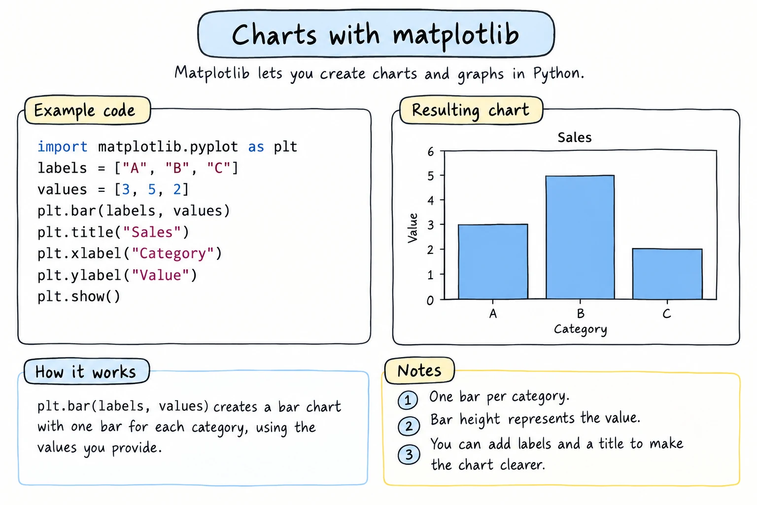
What you'll learn
- How to draw line, bar, histogram, scatter, and pie charts
- How to add titles, axis labels, legends, grids, colors, and markers
- How to put several charts in one figure with
plt.subplots()and the Axes API - How to save a chart as an image file
- How to plot directly from a pandas DataFrame, and how to pick the right chart
Why it matters
A table of 365 daily temperatures tells you very little at a glance. A line chart of the same numbers shows the hot summer, the cold winter, and the one strange week in April instantly. Charts help you find patterns while you explore data, and they help you explain results to other people: a manager, a teacher, or readers of a report.
matplotlib is the classic plotting library for Python. pandas uses it behind the scenes, and many other tools build on it, so the ideas in this lesson carry over widely.
Setup and your first chart
matplotlib is a third-party package. On your own computer, install it with:
python -m pip install pandas matplotlibIn the editor on this site, it loads automatically, and the chart appears below your code when it calls plt.show().
The part of matplotlib you use most is pyplot, imported as plt by convention:
import matplotlib.pyplot as plt

months = ["Jan", "Feb", "Mar", "Apr", "May", "Jun"]
temps = [2, 5, 12, 19, 25, 30]

plt.plot(months, temps)
plt.title("Average temperature in Tashkent")
plt.xlabel("Month")
plt.ylabel("Temperature (°C)")
plt.show()
This draws a single blue line that rises from 2 °C in January to 30 °C in June, with the months along the bottom axis.
plt.plot(x, y) takes the horizontal values first and the vertical values second. plt.show() displays the finished chart. Without it, a script run from a terminal shows nothing.
Two ways to use matplotlib
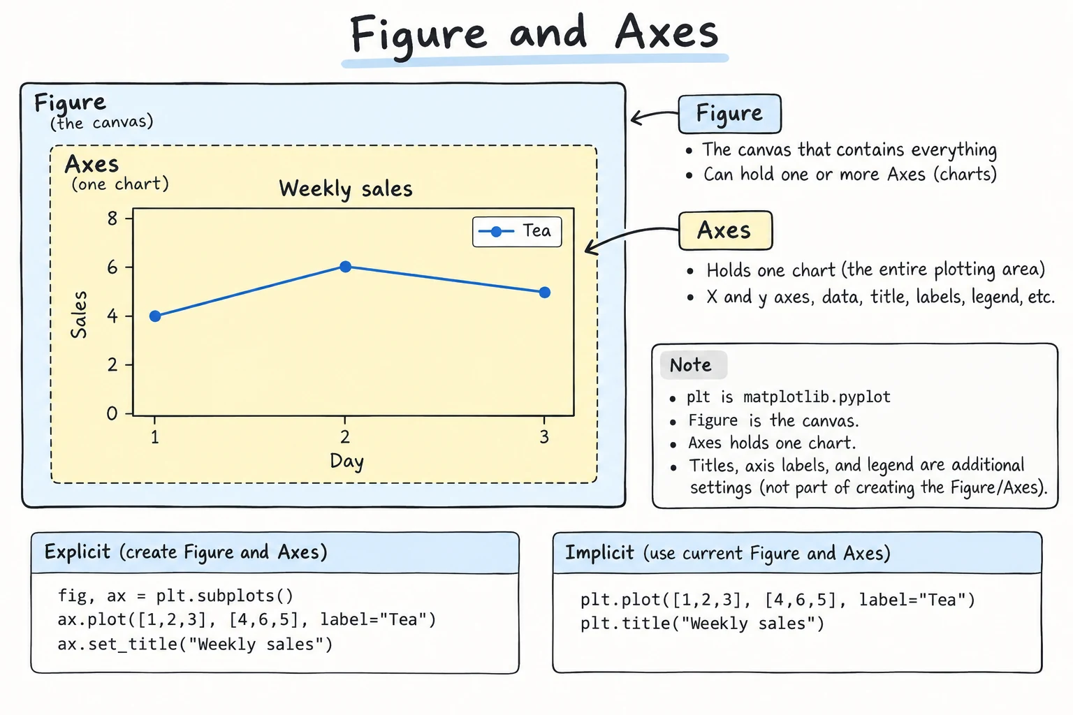
matplotlib has two styles:
| Style | Looks like | Best for |
|---|---|---|
| pyplot style | plt.plot(...), plt.title(...) | quick, single charts |
| object-oriented (Axes) style | fig, ax = plt.subplots(), ax.plot(...), ax.set_title(...) | anything with several charts, functions, or reusable code |
In the object-oriented style, a Figure is the whole image, and an Axes is one chart inside it, with its own axes, title, and data:
The official documentation recommends the Axes style, because it is always clear which chart each command changes. Here is the same chart written that way:
import matplotlib.pyplot as plt

months = ["Jan", "Feb", "Mar", "Apr", "May", "Jun"]
temps = [2, 5, 12, 19, 25, 30]

fig, ax = plt.subplots()
ax.plot(months, temps)
ax.set_title("Average temperature in Tashkent")
ax.set_xlabel("Month")
ax.set_ylabel("Temperature (°C)")
plt.show()
The chart is identical. Notice the name changes: plt.title() becomes ax.set_title(), and plt.xlabel() becomes ax.set_xlabel(). The rest of this lesson uses the Axes style.
Line charts: several lines, colors, markers, legends
Line charts show how something changes over time. Call ax.plot() once per line, give each a label, and call ax.legend() to show the labels:
import matplotlib.pyplot as plt

months = ["Jan", "Feb", "Mar", "Apr", "May", "Jun"]
tashkent = [2, 5, 12, 19, 25, 30]
nukus = [-3, 0, 8, 17, 24, 29]
termez = [5, 8, 15, 22, 28, 33]

fig, ax = plt.subplots()
ax.plot(months, tashkent, marker="o", label="Tashkent")
ax.plot(months, nukus, marker="s", linestyle="--", label="Nukus")
ax.plot(months, termez, marker="^", color="red", label="Termez")

ax.set_title("Average monthly temperature, first half of the year")
ax.set_xlabel("Month")
ax.set_ylabel("Temperature (°C)")
ax.legend()
ax.grid(True, alpha=0.3)
plt.show()
The chart shows three rising lines: Termez (red, triangles) is warmest every month, Nukus (dashed, squares) starts below freezing, and all three converge by June. A faint grid makes values easier to read.
Useful styling arguments:
| Argument | Examples | Effect |
|---|---|---|
color | "red", "tab:green", "#1f77b4" | line or bar color |
marker | "o", "s", "^", "x" | dot shape at each data point |
linestyle | "-", "--", ":" | solid, dashed, dotted |
linewidth | 1, 2.5 | line thickness |
alpha | 0.3 | transparency from 0 to 1 |
Bar charts
Bar charts compare amounts across categories:
import matplotlib.pyplot as plt

cities = ["Tashkent", "Samarkand", "Bukhara", "Fergana"]
revenue = [297, 182, 187, 145]   # thousand som

fig, ax = plt.subplots()
bars = ax.bar(cities, revenue, color="tab:blue")
ax.bar_label(bars)                 # write the value on top of each bar
ax.set_title("Revenue by city, March 2026")
ax.set_xlabel("City")
ax.set_ylabel("Revenue (thousand som)")
plt.show()
The chart shows four vertical bars, with Tashkent clearly the tallest at 297 and Fergana the shortest. ax.bar_label(bars) prints each value above its bar, which saves the reader from estimating heights.
When category names are long or there are many of them, a horizontal bar chart with barh() keeps the labels readable. Sorting the values first makes the ranking obvious:
import matplotlib.pyplot as plt

products = {
    "Green tea": 270,
    "Samsa with meat": 240,
    "Apple juice": 156,
    "Halva": 92,
    "Non (flatbread)": 310,
}
ranked = sorted(products.items(), key=lambda pair: pair[1])
names = [name for name, value in ranked]
values = [value for name, value in ranked]

fig, ax = plt.subplots()
ax.barh(names, values, color="tab:orange")
ax.set_title("Product sales, first quarter")
ax.set_xlabel("Revenue (thousand som)")
fig.tight_layout()
plt.show()
The bars run left to right, sorted so that the best seller, non, sits at the top and halva at the bottom. barh() draws the first item at the bottom, which is why the list is sorted from smallest to largest. fig.tight_layout() makes room for the long product names on the left.
Histograms
A histogram shows how values are spread out: it divides the range into bins and counts how many values fall into each one.
import random
import matplotlib.pyplot as plt

random.seed(42)
scores = [min(100, max(0, round(random.gauss(72, 12)))) for _ in range(200)]

fig, ax = plt.subplots()
ax.hist(scores, bins=10, color="tab:green", edgecolor="black")
ax.set_title("Exam scores of 200 students")
ax.set_xlabel("Score")
ax.set_ylabel("Number of students")
plt.show()
The chart is a hill of bars with its peak between 70 and 80, with fewer students at very low and very high scores. edgecolor draws outlines so neighboring bars do not blend together.
Do not confuse a histogram with a bar chart. A bar chart compares separate categories (cities), while a histogram groups a continuous number (scores) into ranges.
Scatter plots
A scatter plot draws one dot per item and shows the relationship between two numbers:
import matplotlib.pyplot as plt

area = [35, 48, 52, 60, 67, 75, 80, 92, 105, 120]            # square meters
price = [420, 560, 590, 700, 760, 880, 910, 1050, 1180, 1400]  # million som

fig, ax = plt.subplots()
ax.scatter(area, price, color="tab:purple", s=60, alpha=0.7)
ax.set_title("Apartment prices in Tashkent")
ax.set_xlabel("Area (m²)")
ax.set_ylabel("Price (million som)")
ax.grid(True, alpha=0.3)
plt.show()
The dots climb from the bottom left to the top right, showing that bigger apartments cost more in an almost straight line. s sets the dot size.
Pie charts, with a caveat
A pie chart shows parts of a whole:
import matplotlib.pyplot as plt

labels = ["Cash", "Card", "Click", "Payme"]
shares = [35, 30, 20, 15]

fig, ax = plt.subplots()
ax.pie(shares, labels=labels, autopct="%1.0f%%", startangle=90)
ax.set_title("How customers pay")
plt.show()
The chart is a circle cut into four slices labeled with percentages, with cash as the largest slice at 35%. autopct formats the percentage text, and startangle=90 starts the first slice at the top.
Use pie charts sparingly
People are bad at comparing angles. Is the 35% slice visibly bigger than the 30% one? In a bar chart, the difference is obvious. Use a pie only for a few slices (about 2 to 5) that add up to a meaningful whole. Otherwise, use a bar chart.
Several charts in one figure: subplots
plt.subplots(nrows, ncols) creates a grid of Axes. With one row and two columns, you get an array of two Axes that you can unpack:
import matplotlib.pyplot as plt

months = ["Jan", "Feb", "Mar", "Apr", "May", "Jun"]
temps = [2, 5, 12, 19, 25, 30]
rain = [55, 47, 70, 64, 29, 8]

fig, (ax1, ax2) = plt.subplots(1, 2, figsize=(10, 4))

ax1.plot(months, temps, marker="o", color="tab:red")
ax1.set_title("Temperature")
ax1.set_ylabel("°C")

ax2.bar(months, rain, color="tab:blue")
ax2.set_title("Rainfall")
ax2.set_ylabel("mm")

fig.suptitle("Tashkent weather, January to June")
fig.tight_layout()
plt.show()
The figure shows two charts side by side: a red line of rising temperature on the left and blue rainfall bars on the right, which peak in March and nearly vanish by June.
figsize=(10, 4)sets the figure size in inches (width, height).fig.suptitle()adds one title above all the charts.fig.tight_layout()adjusts the spacing so titles and labels do not overlap.
For a grid of 2 rows and 2 columns, use fig, axes = plt.subplots(2, 2) and reach each chart with axes[row, col]: row first, as in the grids from Nested Data, but with both indexes in one pair of brackets.
Saving figures
fig.savefig() writes the chart to an image file. The file type comes from the extension: .png, .jpg, .svg, or .pdf.
from pathlib import Path
import matplotlib.pyplot as plt

cities = ["Tashkent", "Samarkand", "Bukhara"]
visitors = [820, 1240, 960]   # thousand per year

fig, ax = plt.subplots()
ax.bar(cities, visitors)
ax.set_title("Tourist visits per year")
ax.set_ylabel("Visitors (thousands)")

fig.savefig("visitors.png", dpi=150, bbox_inches="tight")
print(Path("visitors.png").exists())Truedpi=150sets the resolution. 100 is fine for screens, and 300 is good for print.bbox_inches="tight"trims extra white space and keeps long labels from being cut off.- Call
savefig()beforeplt.show(). In a script, closing the chart window can leave you saving an empty figure. - When a loop creates many figures (one chart per city, say), call
plt.close(fig)after saving each one, or matplotlib keeps them all in memory and warns you.
Where plt.show() is needed
In a .py file and in this site's editor, plt.show() is what displays the chart (here it appears below the output). In Jupyter and the Python Lab, a figure is shown automatically at the end of a cell, so you can leave plt.show() out.
Plotting straight from pandas
A DataFrame or Series has a .plot() method that calls matplotlib for you. It uses the index for the x-axis and the column names for the legend:
import io
import pandas as pd
import matplotlib.pyplot as plt

text = """city,product,quantity,price
Tashkent,Tea,4,15000
Samarkand,Samsa,10,8000
Tashkent,Juice,3,12000
Bukhara,Tea,5,15000
Tashkent,Samsa,12,8000
Samarkand,Juice,6,12000
Bukhara,Samsa,8,8000
Tashkent,Tea,7,15000
Samarkand,Tea,2,15000
Bukhara,Juice,4,12000
"""
sales = pd.read_csv(io.StringIO(text))
sales["revenue"] = sales["quantity"] * sales["price"]

table = sales.pivot_table(index="city", columns="product",
                          values="revenue", aggfunc="sum")

ax = table.plot(kind="bar", rot=0)
ax.set_title("Revenue by city and product")
ax.set_xlabel("City")
ax.set_ylabel("Revenue (som)")
plt.show()
The chart groups three bars (Juice, Samsa, Tea) for each city, with a legend for the products. Tea in Tashkent is the tallest bar.
kind can be "line", "bar", "barh", "hist", "scatter", or "pie". rot=0 keeps the city names horizontal. Because .plot() returns the Axes, you customize it with the same ax.set_... methods. You can also pass ax= to draw a pandas plot inside a subplot you created yourself.
Choosing the right chart
| You want to show | Use | Example |
|---|---|---|
| change over time | line chart | monthly temperature |
| comparison between categories | bar chart | revenue per city |
| ranking with long names | horizontal bar chart | top products |
| how values are distributed | histogram | exam scores |
| relationship between two numbers | scatter plot | area vs. price |
| parts of a whole (few parts) | pie chart, or a bar chart | payment methods |
When in doubt, start with a bar chart or a line chart. They are the easiest to read.
Try it
Change the data, the colors, or kind="bar" to kind="barh", and run again.
Common mistakes
1. Forgetting plt.show()
import matplotlib.pyplot as plt

fig, ax = plt.subplots()
ax.plot([1, 2, 3], [4, 1, 5])
# Bad: the script ends and no window ever appears
In a script, nothing appears until plt.show() runs. Jupyter notebooks show charts automatically, which is why this mistake often shows up when code moves from a notebook into a .py file.
2. Overlapping labels
Long category names on the x-axis crash into each other:
ax.bar(["Tashkent region", "Samarkand region", "Kashkadarya region"], [30, 25, 18])Fix it by rotating the labels, letting matplotlib fix the spacing, or switching to barh():
ax.tick_params(axis="x", labelrotation=45)   # Good: tilted labels
fig.tight_layout()                           # Good: no clipped labels
3. Numbers without labels or units
fig, ax = plt.subplots()
ax.plot(months, revenue)      # Bad: no title, no axis labels
plt.show()
The reader has to guess: degrees or millimeters? Som or dollars? Always set a title and label both axes, including units: ax.set_ylabel("Revenue (thousand som)"). A pie with a dozen thin slices is just as hard to read: keep the biggest few categories, group the rest into "Other", or use a sorted barh().
4. Mixing plt. and ax. names
import matplotlib.pyplot as plt

fig, ax = plt.subplots()
ax.title("Sales") # Bad: Axes uses set_titleTypeError: 'Text' object is not callableOn an Axes, use the set_ versions: ax.set_title(), ax.set_xlabel(), ax.set_ylabel(). plt.title() has no set_ because it acts on the current chart.
Practice
1. Weekly steps
Aziza tracked her steps for a week. Draw a line chart with markers, the title Aziza's steps this week, and labeled axes. To check your chart, print its title with ax.get_title(), then the number of points on the line and the highest value, read from ax.lines[0].get_ydata().
days = ["Mon", "Tue", "Wed", "Thu", "Fri", "Sat", "Sun"]
steps = [6200, 8400, 7100, 9800, 5600, 12300, 10100]
Solution
import matplotlib.pyplot as plt

days = ["Mon", "Tue", "Wed", "Thu", "Fri", "Sat", "Sun"]
steps = [6200, 8400, 7100, 9800, 5600, 12300, 10100]

fig, ax = plt.subplots()
ax.plot(days, steps, marker="o")
ax.set_title("Aziza's steps this week")
ax.set_xlabel("Day")
ax.set_ylabel("Steps")
ax.grid(True, alpha=0.3)

line_values = ax.lines[0].get_ydata()
print(ax.get_title())
print(len(line_values), "points, peak", max(line_values))
plt.show()Aziza's steps this week
7 points, peak 12300The line dips on Friday and peaks on Saturday at 12,300 steps.
2. Library loans
Draw a horizontal bar chart of book loans by genre, sorted so the most popular genre is at the top. To check your chart, print the genre labels from bottom to top (ax.get_yticklabels(), using each label's get_text()) and the bar lengths (ax.patches, using each bar's get_width()).
loans = {"Poetry": 45, "History": 80, "Science": 62, "Novels": 130, "Children": 95}Solution
import matplotlib.pyplot as plt

loans = {"Poetry": 45, "History": 80, "Science": 62, "Novels": 130, "Children": 95}
ranked = sorted(loans.items(), key=lambda pair: pair[1])

fig, ax = plt.subplots()
ax.barh([genre for genre, n in ranked], [n for genre, n in ranked])
ax.set_title("Library loans by genre")
ax.set_xlabel("Number of loans")

print([label.get_text() for label in ax.get_yticklabels()])
print([int(bar.get_width()) for bar in ax.patches])
plt.show()['Poetry', 'Science', 'History', 'Children', 'Novels']
[45, 62, 80, 95, 130]Novels appear at the top with 130 loans. Sorting from smallest to largest works because barh() draws the first bar at the bottom.
3. Heights histogram and scatter
Using the data below, make a figure with two side-by-side charts: a histogram of heights with 8 bins, and a scatter plot of height (x) against weight (y). Give each chart a title and axis labels, and add the overall title Survey of 100 adults. To check your figure, print the overall title with fig.get_suptitle(), then the number of histogram bars (ax1.patches) and scatter points (ax2.collections[0].get_offsets()).
import random

random.seed(7)
heights = [round(random.gauss(170, 8), 1) for _ in range(100)]
weights = [round(h * 0.9 - 88 + random.gauss(0, 6), 1) for h in heights]
Solution
import random
import matplotlib.pyplot as plt

random.seed(7)
heights = [round(random.gauss(170, 8), 1) for _ in range(100)]
weights = [round(h * 0.9 - 88 + random.gauss(0, 6), 1) for h in heights]

fig, (ax1, ax2) = plt.subplots(1, 2, figsize=(10, 4))

ax1.hist(heights, bins=8, edgecolor="black")
ax1.set_title("Height distribution")
ax1.set_xlabel("Height (cm)")
ax1.set_ylabel("People")

ax2.scatter(heights, weights, alpha=0.6)
ax2.set_title("Height vs. weight")
ax2.set_xlabel("Height (cm)")
ax2.set_ylabel("Weight (kg)")

fig.suptitle("Survey of 100 adults")
fig.tight_layout()

print(fig.get_suptitle())
print(len(ax1.patches), "bars,", len(ax2.collections[0].get_offsets()), "points")
plt.show()Survey of 100 adults
8 bars, 100 pointsThe histogram shows that most heights fall between 160 and 180 cm, and the scatter plot slopes upward: taller people tend to weigh more.
4. Save a chart
Draw a bar chart of the number of students in each group, save it as groups.png with dpi=200 and a tight bounding box, then print whether the saved file is larger than 0 bytes.
groups = ["A", "B", "C", "D"]
students = [24, 28, 19, 26]
Solution
from pathlib import Path
import matplotlib.pyplot as plt

groups = ["A", "B", "C", "D"]
students = [24, 28, 19, 26]

fig, ax = plt.subplots()
ax.bar(groups, students, color="tab:cyan")
ax.set_title("Students per group")
ax.set_xlabel("Group")
ax.set_ylabel("Students")

fig.savefig("groups.png", dpi=200, bbox_inches="tight")
print(Path("groups.png").stat().st_size > 0)True5. Mini sales dashboard
Using the sales data below and pandas, build a figure with two subplots side by side:
- a bar chart of total revenue per city, sorted from highest to lowest
- a line chart of total revenue per month, with markers
Give each chart a title and axis labels, add an overall title, and use tight_layout().
date,city,quantity,price
2026-01-05,Tashkent,4,15000
2026-01-12,Samarkand,10,8000
2026-01-20,Bukhara,3,12000
2026-02-03,Bukhara,5,15000
2026-02-14,Tashkent,12,8000
2026-02-21,Samarkand,6,12000
2026-03-02,Bukhara,8,8000
2026-03-10,Tashkent,7,15000
2026-03-18,Samarkand,2,15000
2026-04-06,Tashkent,9,12000
2026-04-15,Samarkand,11,8000
2026-04-25,Bukhara,6,15000
Solution
import io
import pandas as pd
import matplotlib.pyplot as plt

text = """date,city,quantity,price
2026-01-05,Tashkent,4,15000
2026-01-12,Samarkand,10,8000
2026-01-20,Bukhara,3,12000
2026-02-03,Bukhara,5,15000
2026-02-14,Tashkent,12,8000
2026-02-21,Samarkand,6,12000
2026-03-02,Bukhara,8,8000
2026-03-10,Tashkent,7,15000
2026-03-18,Samarkand,2,15000
2026-04-06,Tashkent,9,12000
2026-04-15,Samarkand,11,8000
2026-04-25,Bukhara,6,15000
"""
sales = pd.read_csv(io.StringIO(text), parse_dates=["date"])
sales["revenue"] = sales["quantity"] * sales["price"] / 1000   # thousand som

by_city = sales.groupby("city")["revenue"].sum().sort_values(ascending=False)
by_month = sales.groupby(sales["date"].dt.month)["revenue"].sum()
print(by_city)
print(by_month)

fig, (ax1, ax2) = plt.subplots(1, 2, figsize=(11, 4))

ax1.bar(by_city.index, by_city.values, color="tab:blue")
ax1.set_title("Revenue by city")
ax1.set_xlabel("City")
ax1.set_ylabel("Revenue (thousand som)")

ax2.plot(by_month.index, by_month.values, marker="o", color="tab:green")
ax2.set_title("Revenue by month")
ax2.set_xlabel("Month")
ax2.set_ylabel("Revenue (thousand som)")
ax2.set_xticks(by_month.index)
ax2.grid(True, alpha=0.3)

fig.suptitle("Sales dashboard, January to April 2026")
fig.tight_layout()
plt.show()city
Tashkent 369.0
Samarkand 270.0
Bukhara 265.0
Name: revenue, dtype: float64
date
1 176.0
2 243.0
3 199.0
4 286.0
Name: revenue, dtype: float64The left chart ranks the cities, with Tashkent first, and the right chart shows monthly revenue rising in February, dipping in March, and reaching its highest point in April. set_xticks() makes the month axis show only whole month numbers. The groupby results are Series, so .index gives the labels and .values gives the numbers to plot.
Recap
- Import with
import matplotlib.pyplot as plt, draw, and finish withplt.show(). - Prefer the Axes style:
fig, ax = plt.subplots(), thenax.plot(),ax.bar(),ax.barh(),ax.hist(),ax.scatter(), orax.pie(). - Always add a title and axis labels with units. Use
label=plusax.legend()for several series. plt.subplots(rows, cols, figsize=...)builds grids of charts, andfig.tight_layout()fixes overlaps.- Save with
fig.savefig("chart.png", dpi=150, bbox_inches="tight")before showing, andplt.close(fig)in loops; pandas objects plot directly with.plot(kind=...). - Match the chart to the question: line for time, bar for categories, histogram for distributions, scatter for relationships, pie only for a few parts of a whole.